Kernel Density Estimation (Dynamic Heatmap)

Author:

Thomas Bonfort, Mathieu Coudert

Contact:

tbonfort at terriscope.fr, mathieu.coudert at gmail.com

Last Updated:

2014/11/02

Introduction

Added in version 7.0.

A heatmap is a popular method for representing sparse data on a regular raster grid, where each pixel on the grid is influenced inversely to its distance to each sample of the sparse dataset. Heatmaps are usually represented with a color-ramp where the hue encodes the density of the data sample, optionally along with the intensity of an attribute. The "heatmap" term itself is used with varying meanings. We will be using it to reference Kernel Density Estimation maps.

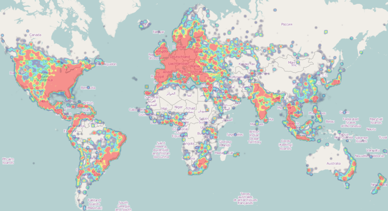
Example Kernel Density Estimation Map (image cc-by-sa wikipedia)

Configuration

First, you must set the LAYER CONNECTIONTYPE parameter to KERNELDENSITY. The heatmap vector-to-raster takes the following parameters:

• CONNECTION "layername" : reference to the NAME or GROUP of a LAYER to use as an input vector datasource. NAME takes precedence, followed by the first layer from GROUP who's minscaledenom/maxscaledenom matches the current map scale. The referenced layer should be a TYPE POINT layer. Other layer types will result in one sample being added for each vertex of the input features.

• PROCESSING "KERNELDENSITY_RADIUS=10" : radius in pixels of the gaussian filter to apply to the bitmap array once all features have been accumulated. Higher values result in increased cpu time needed to compute the filtered data.

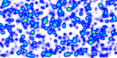
Result with kerneldensity_radius set to 10 (pixels)

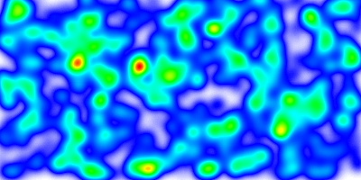
Result with kerneldensity_radius set to 20 (pixels)

• PROCESSING "KERNELDENSITY_COMPUTE_BORDERS=ON|OFF" : A kernel of radius "r" cannot be applied to "r" pixels along the borders of the image. The default is to extend the search rectangle of the input datasource to include features "r" pixels outside of the current map extent so that the computed heatmap extends to the full extent of the resulting image. This can be deactivated when tiling if the tiling software applies a metabuffer of "r" pixels to its requests, to avoid the performance overhead of computing this extra information.

• PROCESSING "KERNELDENSITY_NORMALIZATION=AUTO|numeric" : If set to "AUTO", the created raster band will be scaled such that its intensities range from 0 to 255, in order to fully span the configured color ramp. Such behavior may not be desirable (typically for tiling) as the resulting intensity of a pixel at a given location will vary depending on the extent of the current map request. If set to a numeric value, the samples will be multiplied by the given value. It is up to the user to determine which scaling value to use to make the resulting pixels span the full 0-255 range; determining that value is mostly a process of trial and error. Pixels that fall outside the 0-255 range will be clipped to 0 or 255.

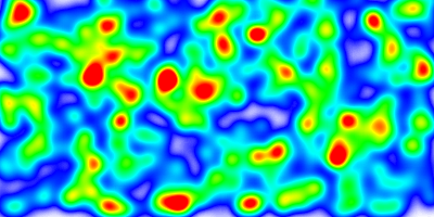
Fixed scaling applied. Compared to the previous images, the greater number of red areas results from the fact that the chosen scaling factor made a large number of pixels overshoot the 255 limit.

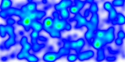
Lower fixed scaling applied. No pixels have attained the 255 limit.

Advanced sample weighting and filtering

By default, each feature is assigned a weight of 1.0, and the resulting heatmap will represent the spatial density of the vector features. If this is not the desired behavior, different weights can be applied on a feature by feature basis by using regular CLASS / STYLE syntax on the source vector layer. The weight used will be read from the SIZE value of the matched STYLE. Standard EXPRESSION and MINSCALEDENOM / MAXSCALEDENOM apply; if a feature results in no matching CLASS and/or STYLE, it is ignored and discarded from the resulting heatmap. The examples at the end give some examples as to how this can be achieved.

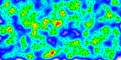
Heatmap representing pure feature density when sample weighting or filtering is not applied, the actual vector points are represented alongside. (The other examples are rendered with attribute weighting on each sample)

Raster Color Ramping

The features added in MS RFC 6: Color Range Mapping of Continuous Feature Values for vector features, and since extended to support raster layers, will be extended in order to support more complex color ramps. Note that these additions will apply to all raster classifications, not only for heatmap layers.

• Support for multiple stops : The actual support for ranges for raster layers is limited to a single COLORRANGE / DATARANGE. We will support multiple ranges in order to allow multiple color stops, and will also account for optional alpha values. The following example creates a ramp ranging from fully transparent blue to blue for values between 0 and 32, then blue to red for values ranging from 32 to 255.

  CLASS
    STYLE
      COLORRANGE  "#0000ff00"  "#0000ffff"
      DATARANGE 0 32
    END # STYLE
    STYLE
      COLORRANGE  "#0000ffff"  "#ff0000ff"
      DATARANGE 32 255
    END # STYLE
  END # CLASS
  

  Catatan

  A single style block will be used for each pixel value. It is up to the user to ensure that the supplied DATARANGE`s span 0 to 255 with no overlap, and that the chosen `COLORRANGE stops are continuous from one stop to the next.

• PROCESSING RANGE_COLORSPACE=RGB|HSL: The current RANGE support interpolates colors between stops in RGB space, which usually results in washed out colors. The interpolation can be done in HSL space which usually results in wanted output for heatmaps.

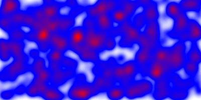
washed out colors when interpolating in RGB space.

Example mapfiles

MAP
  SIZE 1000 500
  EXTENT -180 -90 180 90
  NAME "test heat"
  IMAGETYPE "png"

  WEB
    METADATA
      "ows_srs" "epsg:4326  epsg:3857 epsg:900913"
      "ows_enable_request" "*"
    END # METADATA
  END # WEB

  PROJECTION
    "+init=epsg:4326"
  END # PROJECTION

  LAYER
    NAME "heatmap"
    TYPE raster
    CONNECTIONTYPE kerneldensity
    CONNECTION "points"
    STATUS on
    PROCESSING "RANGE_COLORSPACE=HSL"
    PROCESSING "KERNELDENSITY_RADIUS=20"
    PROCESSING "KERNELDENSITY_COMPUTE_BORDERS=ON"
    PROCESSING "KERNELDENSITY_NORMALIZATION=AUTO"
    OFFSITE 0 0 0
    CLASS
      STYLE
        COLORRANGE  "#0000ff00"  "#0000ffff"
        DATARANGE 0 32
      END # STYLE
      STYLE
        COLORRANGE  "#0000ffff"  "#ff0000ff"
        DATARANGE 32 255
      END # STYLE
    END # CLASS
  END # LAYER

  LAYER
      NAME "points"
      STATUS on
      TYPE POINT
      DATA "pnts.shp"
   END # LAYER
END # MAPFILE

The kernel radius can be set dynamically depending on the scale. Note that any other PROCESSING key can be updated by the same method. In the following example, the kernel radius will be 50 pixels for scales 1/1 to 1/25000000, and 10 pixels for scales 1/25000000 and smaller:

LAYER
  NAME "heatmap"
  ...
  PROCESSING "KERNELDENSITY_RADIUS=%radius%"
  SCALETOKEN
    NAME "%radius%"
    VALUES
      "0" "50"
      "25000000" "10"
    END # VALUES
  END # SCALETOKEN
  ...
END # LAYER

Different weights can be applied by using CLASS->`STYLE`->`SIZE` syntax on the source vector layer to apply a non default weight to each sample:

• Weight read from a feature attribute:

  LAYER
    NAME "points"
    STATUS on
    TYPE POINT
    DATA "pnts.shp"
    CLASS
      STYLE
        SIZE [attribute]
      END # STYLE
    END # CLASS
  END # LAYER
  

• Weight read from a non numeric attribute:

  LAYER
    NAME "points"
    STATUS on
    TYPE point
    DATA "pnts.shp"
    CLASSITEM "risk"
    CLASS
      EXPRESSION "high"
      STYLE
        SIZE 5
      END # STYLE
    END # CLASS
    CLASS
      EXPRESSION "medium"
      STYLE
        SIZE 3
      END # STYLE
    END # CLASS
    CLASS
      EXPRESSION "low"
      STYLE
        SIZE 1
      END # STYLE
    END # CLASS
  END # LAYER